Methodology and Study Procedere of the Mannheim Corona Study

The Mannheim Corona Study is based on the methodology and infrastructure of the German Internet Panel (GIP). Like the GIP, the Mannheim Corona Study was led by Prof. Dr. Blom and conducted by the GIP team. The questionnaires were developed together with the researchers at the Collaborative Research Center (SFB) 884 “Political Economy of Reforms”.

Study Procedere

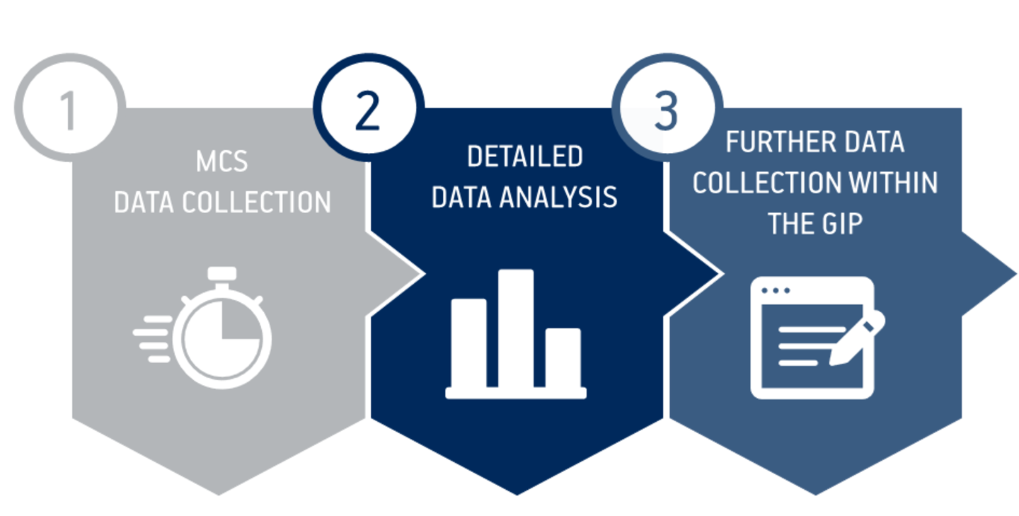
Phase 1: Data Collection

In the data collection phase of the Mannheim Corona Study, approximately 3,600 participants of the German Internet Panel (GIP) were interviewed every week from 20 March to 10 July 2020 about how their lives have changed since the Corona crisis. We examined socio-economic aspects (e.g. childcare, work situations, and disposable income) as well as the influence of political measures on social interactions, fears and the social acceptance of measures to contain the pandemic. The study participants were evenly distributed over the days of the week so that we gained daily insights into the developments of the population.

Phase 2: Detailed Data Analyses

The data collected during the 16 weeks of the MCS are the basis for the second phase, in which we conduct detailed analyses and draw further conclusions about the effects of the pandemic in Germany. As the Mannheim Corona Study is a panel study that builds on an existing long-term study, this allows us to compare life in Germany before and since the outbreak. The interviewed panel members have regularly participated in our study for at least 18 months before entering the MCS; some participants have been part of the GIP for 8 years.

Phase 3: Further Data Collection

By integrating the MCS into the ongoing data collection of the GIP, the long-term consequences of the Corona pandemic for Germany can also be investigated in the third phase of the study.

The random sample of the GIP from the registers of the residents' registration offices throughout Germany and our two-stage weighting procedure allows the Mannheim Corona Study to draw conclusions about the general population in Germany. In contrast to many short-term studies that rely on commercial online respondent pools, the representativeness of the Mannheim Corona Study is statistically supported.

Study Methodology

Sample
The sample of the Mannheim Corona Study was divided into eight random sub-samples. The sub-samples 1–7 were assigned to a specific day of the week, while the eighth sub-sample served as control group and was not surveyed for the Corona Study.
Organisation of the Daily Surveys
On each day of the week one of the sub-samples received an email invitation to the day’s survey. Contacted panel members had 48 hours to participate. However, they were encouraged to take part on the day of the week that they were assigned to, i.e. within the first 24 hours.
Results for each day are analyzed together, i.e. persons who responded directly on the first day (e.g. Monday) are included in the analysis of that specific day (Monday). Answers of respondents who participated on the day after (Tuesday) are analyzed together with the answers on that day of the next sub-sample. In this way, we minimize biases, because every daily analysis includes both early as well as late respondents.
Within one week, the questionnaire remains exactly the same for all participants. Across weeks, we also aimed to keep the questionnaires constant to allow for a daily continuation of our time series for a long time. However, to conduct in-depth analyses of selected topics and to react to unforeseen events, the questionnaire was evaluated and updated every week.
Weighting and Representativeness
No serious academic study in the field of social and economic research will generally claim to be representative of the population. While commercial research institutes tend to emphasize their representativeness, academia usually tries to avoid the use of this term.
Of course, high-quality academic studies go through great lengths to come as close as possible to ideal of representativeness. To this end, researchers use random samples, elaborate fieldwork procedures, and scientific weighting algorithms to represent the general population as closely as possible across a variety of population statistics. The Mannheim Corona Study in the German Internet Panel is also committed to this professional ethos.
For general information on the GIP sampling strategy and its implementation, please visit our site methodology.
The analyses conducted with the Mannheim Corona Study are weighted with a carefully calculated weight. For this purpose, we carried out a two-stage weighting procedure:
In the first stage, we calculated a response propensity weight, which projects the characteristics of the Corona Study participants to the general GIP study. This included two characteristics: employment and occupational sector.
In the second stage, a raking weight was estimated. This raking weight extrapolated the characteristics of Corona Study participants to those of the general population of Germany (based on the German Mikrozensus). The following characteristics informed the raking procedure: age, gender, marital status, highest level of education, household size, and federal state.
A chained equation algorithm imputed missing values in the weighting variables. The final weight was trimmed for values > 4 and values < 1/4.
Funding
The Mannheim Corona Study is conducted within the GIP at the Collaborative Research Center (SFB) 884 “Political Economy of Reforms” and funded by the German Research Foundation (DFG). All researchers involved are part of the SFB 884 and mostly funded by the DFG. Neither the Mannheim Corona Study nor the GIP pursue economic or political interests of any kind.

Further publications

A methodological analysis of the MCS was published in the Survey Research Methods special issue on survey research methods during the COVID-19 crisis. The article and appendix tables can be found below.

Methodological Results

Week	Mon	Tue	Wed	Thu	Fri	Sat	Sun	Total
1	62.8%	59.4%	64.5%	60.4%	56.8%	57.8%	59.5%	60.2%
2	68.7%	61.0%	67.6%	63.5%	60.8%	63.0%	66.1%	64.4%
3	66.2%	61.1%	66.1%	62.5%	60.2%	63.1%	65.9%	63.6%
4	67.0%	61.6%	66.0%	63.4%	59.3%	59.3%	63.1%	62.8%
5	66.7%	61.5%	64.3%	62.9%	61.2%	62.5%	65.9%	63.6%
6	66.2%	60.4%	65.5%	63.9%	57.6%	62.8%	65.3%	63.1%
7	64.8%	57.5%	61.8%	60.1%	58.8%	61.3%	64.1%	61.2%
8	65.0%	58.4%	64.4%	61.8%	57.8%	60.3%	66.4%	62.0%
9	64.2%	57.6%	60.0%	59.6%	60.5%	60.8%	63.6%	60.9%
10	65.7%	56.5%	62.8%	61.4%	60.2%	62.0%	62.9%	61.6%
11	60.2%	56.8%	63.0%	61.3%	56.1%	59.5%	60.1%	59.6%
12	61.3%	55.1%	62.4%	58.0%	59.4%	59.1%	62.0%	59.6%
13	61.3%	57.1%	63.5%	59.3%	56.8%	58.6%	64.6%	60.2%
14	61.7%	52.8%	60.6%	58.4%	58.4%	57.5%	60.4%	58.5%
15	62.2%	53.8%	58.9%	57.6%	54.4%	58.9%	62.0%	58.3%
16	61.1%	53.0%	59.8%	57.3%	54.7%	56.1%	61.3%	57.6%
Total	64.1%	57.7%	63.2%	60.7%	58.3%	60.1%	63.3%	61.1%

Week	Mon	Tue	Wed	Thu	Fri	Sat	Sun	Total
1	56.2%	52.1%	56.0%	52.6%	45.9%	45.9%	51.3%	50.9%
2	62.8%	54.8%	60.9%	57.5%	53.7%	50.3%	58.0%	56.8%
3	59.2%	55.5%	58.4%	55.4%	53.1%	51.6%	57.1%	55.8%
4	57.3%	55.4%	58.8%	55.5%	51.8%	47.9%	52.3%	54.1%
5	61.0%	53.6%	57.3%	54.3%	53.7%	50.0%	58.4%	55.4%
6	57.8%	53.5%	58.4%	57.6%	50.4%	51.5%	56.6%	55.1%
7	59.2%	49.8%	53.0%	51.5%	48.6%	50.4%	56.1%	52.6%
8	58.1%	52.0%	57.1%	56.3%	49.2%	47.5%	56.3%	53.8%
9	55.8%	51.6%	52.7%	48.1%	51.1%	48.9%	53.1%	51.6%
10	59.7%	49.9%	54.9%	54.5%	51.1%	49.9%	41.7%	51.7%
11	51.1%	48.0%	56.4%	55.5%	49.2%	46.6%	48.8%	50.8%
12	52.2%	48.4%	54.9%	50.6%	49.4%	44.6%	48.2%	49.8%
13	54.6%	50.4%	54.9%	50.5%	48.1%	46.3%	56.7%	51.6%
14	55.4%	46.4%	53.1%	51.2%	48.8%	43.9%	52.6%	50.2%
15	56.2%	48.2%	50.7%	50.2%	47.8%	45.5%	52.9%	50.2%
16	52.7%	44.6%	53.1%	50.2%	45.6%	42.3%	51.4%	48.6%
Total	56.8%	50.9%	55.7%	53.2%	49.8%	47.7%	53.2%	52.5%

Week	Mon	Tue	Wed	Thu	Fri	Sat	Sun	Total
1	89.4%	87.8%	86.8%	87.2%	80.8%	79.4%	86.1%	85.4%
2	91.4%	89.8%	90.0%	90.6%	88.3%	79.8%	87.7%	88.2%
3	89.4%	90.8%	88.3%	88.6%	88.1%	81.8%	86.7%	87.7%
4	85.6%	89.9%	89.0%	87.6%	87.3%	80.8%	82.8%	86.1%
5	91.4%	87.2%	89.1%	86.3%	87.7%	80.0%	88.6%	87.2%
6	87.3%	88.6%	89.1%	87.4%	87.6%	82.1%	86.8%	87.0%
7	91.3%	86.5%	85.8%	85.7%	82.6%	82.2%	87.5%	86.0%
8	89.4%	89.1%	88.7%	91.1%	85.1%	78.8%	84.7%	86.7%
9	86.9%	89.6%	87.9%	80.7%	84.5%	80.5%	83.5%	84.8%
10	90.9%	88.3%	87.5%	88.8%	84.8%	80.4%	66.4%	83.8%
11	84.8%	84.6%	89.5%	90.6%	87.7%	78.4%	81.1%	85.3%
12	85.1%	87.8%	88.0%	87.3%	83.2%	75.5%	77.8%	83.5%
13	89.0%	88.2%	86.4%	85.2%	84.6%	78.9%	87.8%	85.8%
14	89.9%	87.9%	87.6%	87.8%	83.5%	76.3%	87.2%	85.8%
15	90.3%	89.8%	86.2%	87.2%	87.8%	77.3%	85.3%	86.2%
16	86.3%	84.2%	88.9%	87.8%	83.3%	75.3%	83.9%	84.3%
Total	88.7%	88.1%	88.1%	87.7%	85.4%	79.2%	84.0%	85.9%

	Mon	Tue	Wed	Thu	Fri	Sat	Sun	Total	MZ
Gender
Male	49.6%	49.4%	49.8%	48.9%	51.1%	50.6%	50.6%	50.0%	50.4%
Female	50.4%	50.6%	50.2%	51.1%	48.9%	49.4	49.4%	50.0%	49.6%
Age
16–29	17.3%	16.9%	16.9%	20.0%	16.2%	18.5%	15.2%	17.3%	20.9%
30–39	17.3%	18.7%	17.4%	15.7%	19.1%	17.0%	17.9%	17.6%	16.9%
40–49	13.4%	12.7%	14.7%	14.9%	14.7%	16.2%	15.8%	14.6%	17.4%
50–59	25.0%	25.5%	24.6%	23.6%	25.3%	26.8%	23.3%	24.9%	21.5%
60–75	27.1%	26.2%	26.3%	25.8%	24.7%	21.5%	27.7%	25.6%	23.3%
Education
Low	23.9%	26.6%	26.6%	25.1%	27.2%	26.5%	28.1%	26.3%	31.0%
Medium	35.3%	32.0%	31.4%	30.4%	31.3%	32.8%	32.4%	32.2%	34.0%
High	40.8%	41.4%	42.0%	44.6%	41.5%	40.7%	39.5%	41.5%	35.1%
Household size
1	21.4%	19.7%	22.3%	22.3%	20.8%	20.0%	20.0%	20.9%	21.9%
2	36.4%	37.5%	37.5%	37.1%	35.3%	37.9%	39.3%	37.3%	36.1%
3	18.7%	21.9%	19.3%	18.7%	19.7%	18.6%	21.2%	19.7%	18.8%
4 or more	23.5%	20.9%	21.0%	22.0%	24.2%	23.6%	19.6%	22.1%	23.2%
Citizenship
German	95.0%	97.6%	96.9%	97.1%	97.7%	95.8%	98.6%	97.0%	87.2%
Non-German	5.0%	2.4%	3.1%	2.9%	2.3%	4.2%	1.4%	3.0%	12.8%
Marital status
Single	34.6%	34.5%	35.7%	35.3%	36.6%	36.6%	35.2%	35.5%	35.9%
Married	52.5%	52.4%	50.9%	52.2%	53.0%	52.7%	53.0%	52.4%	52.3%
Other	12.9%	13.1%	13.4%	12.4%	10.4%	10.7%	11.8%	12.1%	11.8%
Region
West	79.5%	80.3%	80.7%	80.3%	80.6%	81.6%	81.4%	80.6%	80.5%
East	20.5%	19.7%	19.3%	19.7%	19.4%	18.4%	18.6%	19.4%	19.5%

	Week 1	Week 2	Week 3	Week 4	Week 5	Week 6	Week 7	Week 8	Week 9	Week 10	Week 11	Week 12	Week 13	Week 14	Week 15	Week 16	Total	MZ
Gender
Male	50.3%	49.6%	50.0%	49.7%	50.6%	49.4%	50.0%	50.0%	50.1%	49.9%	50.1%	50.1%	49.9%	50.5%	50.1%	49.6%	50.0%	50.4%
Female	49.7%	50.4%	50.0%	50.3%	49.4%	50.6%	50.0%	50.0%	49.9%	50.1%	49.9%	49.9%	50.1%	49.5%	49.9%	50.4%	50.0%	49.6%
Age
16–29	17.4%	17.0%	17.5%	16.8%	17.8%	17.0%	17.3%	17.5%	17.5%	17.3%	17.2%	17.8%	17.3%	17.1%	17.5%	17.1%	17.3%	20.9%
30–39	17.5%	17.8%	17.6%	17.7%	17.5%	17.4%	17.5%	18.0%	17.8%	17.7%	17.1%	17.4%	17.3%	17.9%	17.4%	17.5%	17.6%	16.9%
40–49	14.3%	14.9%	14.8%	14.7%	14.6%	14.8%	15.1%	14.3%	14.5%	14.6%	14.6%	14.4%	14.9%	14.6%	14.1%	14.5%	14.6%	17.4%
50–59	25.3%	24.7%	24.5%	24.8%	24.5%	24.5%	24.5%	24.7%	25.2%	25.0%	25.3%	24.7%	24.6%	24.8%	25.1%	25.1%	24.8%	21.5%
60–75	25.5%	25.6%	25.6%	25.9%	25.6%	26.4%	25.6%	25.5%	25.7%	25.4%	25.7%	25.7%	26.0%	25.6%	25.9%	25.8%	25.7%	23.3%
Education
Low	25.8%	26.5%	26.0%	26.4%	26.1%	26.0%	26.6%	26.1%	26.0%	26.6%	26.7%	26.2%	26.2%	26.5%	26.4%	26.0%	26.2%	31.0%
Medium	32.8%	31.8%	32.4%	32.4%	32.0%	32.7%	31.9%	32.3%	33.1%	31.7%	32.6%	32.2%	32.2%	32.2%	32.0%	32.6%	32.3%	34.0%
High	41.4%	41.7%	41.6%	41.2%	41.9%	41.4%	41.5%	41.6%	40.9%	41.7%	40.7%	41.6%	41.6%	41.4%	41.7%	41.5%	41.5%	35.1%
Household size
1	20.9%	21.2%	21.1%	21.0%	20.4%	21.1%	20.7%	20.7%	20.8%	20.5%	21.0%	21.1%	21.0%	21.3%	20.8%	21.2%	20.9%	21.9%
2	37.4%	37.1%	37.0%	37.5%	37.4%	37.6%	37.0%	37.2%	37.6%	37.3%	37.6%	37.1%	37.0%	36.9%	37.6%	37.2%	37.3%	36.1%
3	19.3%	19.4%	19.6%	19.3%	19.8%	19.2%	19.8%	20.1%	19.8%	20.1%	19.7%	19.7%	20.2%	19.9%	20.1%	19.9%	19.7%	18.8%
4 or more	22.4%	22.2%	22.4%	22.2%	22.4%	22.1%	22.5%	21.9%	21.8%	22.1%	21.7%	22.1%	21.8%	21.9%	21.4%	21.7%	22.0%	23.2%
Citizenship
German	96.9%	96.9%	96.6%	97.0%	97.1%	96.8%	97.1%	96.9%	96.8%	97.0%	97.0%	97.1%	97.0%	97.2%	96.8%	97.2%	96.9%	87.2%
Non-German	3.1%	3.1%	3.4%	3.0%	2.9%	3.2%	2.9%	3.1%	3.2%	3.0%	3.0%	2.9%	3.0%	2.8%	3.2%	2.8%	3.1%	12.8%
Marital status
Single	35.7%	35.5%	35.6%	35.2%	35.8%	35.4%	35.3%	35.6%	35.1%	35.6%	35.5%	35.5%	35.3%	35.5%	35.6%	35.1%	35.5%	35.9%
Married	52.3%	52.5%	52.4%	52.4%	52.3%	52.4%	52.6%	52.3%	52.8%	52.3%	52.4%	52.1%	52.4%	52.1%	52.3%	52.6%	52.4%	52.3%
Other	11.9%	12.0%	12.0%	12.4%	11.9%	12.2%	12.1%	12.2%	12.1%	12.2%	12.1%	12.4%	12.4%	12.4%	12.1%	12.4%	12.2%	11.8%
Region
West	80.4%	80.2%	80.6%	80.5%	80.5%	80.7%	80.8%	80.3%	81.0%	80.9%	80.7%	80.5%	80.7%	80.6%	80.4%	80.7%	80.6%	80.5%
East	19.6%	19.8%	19.4%	19.5%	19.5%	19.3%	19.2%	19.7%	19.0%	19.1%	19.3%	19.5%	19.3%	19.4%	19.6%	19.3%	19.4%	19.5%

Week	Mon	Tue	Wed	Thu	Fri	Sat	Sun	Total
1	10.9%	12.0%	11.4%	12.0%	13.2%	11.9%	12.4%	12.0%
2	10.7%	13.6%	11.0%	10.5%	11.5%	9.8%	11.5%	11.2%
3	10.0%	12.6%	10.8%	11.0%	10.9%	8.6%	13.1%	11.0%
4	10.9%	10.7%	10.7%	10.9%	13.1%	9.2%	12.6%	11.5%
5	9.9%	14.0%	10.8%	10.4%	13.7%	11.4%	12.7%	11.8%
6	10.6%	12.6%	12.1%	11.1%	10.8%	10.7%	11.3%	11.3%
7	10.6%	14.6%	10.4%	10.3%	11.4%	11.9%	13.5%	11.8%
8	11.7%	13.5%	11.7%	10.8%	10.2%	10.0%	12.3%	11.5%
9	11.6%	13.8%	12.1%	9.4%	12.4%	9.8%	13.1%	11.7%
10	9.3%	14.9%	11.0%	10.6%	12.7%	10.9%	13.3%	11.8%
11	10.6%	14.8%	10.6%	11.7%	12.7%	11.4%	12.1%	12.0%
12	12.0%	12.9%	10.6%	12.3%	11.8%	10.4%	10.1%	11.5%
13	11.2%	11.9%	11.5%	13.4%	13.1%	8.6%	13.1%	11.8%
14	10.3%	13.0%	13.0%	10.7%	11.9%	9.5%	12.7%	11.6%
15	11.0%	13.2%	13.0%	10.0%	12.3%	10.6%	12.4%	11.8%
16	12.4%	13.6%	11.2%	11.5%	13.0%	10.5%	12.1%	12.0%
Total	10.9%	13.4%	11.4%	11.0%	12.2%	10.3%	12.4%	11.7%

Week	Mon	Tue	Wed	Thu	Fri	Sat	Sun	Total
1	12.0%	12.0%	13.4%	11.2%	11.9%	14.8%	12.0%	12.5%
2	11.6%	13.3%	12.2%	10.3%	12.3%	10.7%	12.7%	11.9%
3	11.3%	13.2%	12.2%	9.9%	10.5%	9.6%	12.5%	11.3%
4	10.9%	14.0%	11.6%	11.0%	13.5%	11.2%	12.2%	12.1%
5	10.5%	15.1%	12.1%	11.6%	13.0%	11.8%	12.9%	12.4%
6	10.7%	14.3%	12.8%	12.1%	10.8%	10.7%	12.2%	11.9%
7	11.8%	14.7%	11.7%	11.3%	10.9%	12.7%	12.0%	12.2%
8	10.9%	14.3%	12.0%	11.0%	11.0%	10.4%	13.0%	11.8%
9	10.8%	14.8%	11.0%	11.5%	12.2%	10.9%	12.7%	12.0%
10	10.8%	15.0%	12.4%	11.6%	12.8%	11.3%	12.8%	12.4%
11	10.4%	13.6%	10.5%	12.3%	12.1%	11.6%	14.6%	12.2%
12	10.2%	16.3%	12.9%	10.7%	11.8%	10.5%	12.6%	12.1%
13	10.7%	12.3%	14.3%	12.3%	11.0%	10.4%	12.0%	11.9%
14	10.3%	15.3%	12.6%	11.5%	13.3%	10.8%	14.2%	12.6%
15	11.9%	13.4%	12.1%	11.5%	13.0%	10.3%	13.7%	12.3%
16	11.5%	14.7%	13.0%	11.7%	13.3%	9.7%	13.9%	12.6%
Total	11.0%	14.1%	12.3%	11.3%	12.1%	11.1%	12.9%	12.1%

Methodology and Study Procedere of the Mannheim Corona Study

Study Procedere

Phase 1: Data Collection

Phase 2: Detailed Data Analyses

Phase 3: Further Data Collection

Study Methodology

Sample

Organisation of the Daily Surveys

Weighting and Representativeness

Funding

Further publications

Methodological Results

Weekly Response Rates

Weekly on the day of invitation response rates

Share of respondents who respond on the day they are invited (rather than the following day)

Socio-demographic composition of MCS respondents by day of the week (averaged across data collection weeks) compared to the German Mikrozensus (weighted data, all characteristics measured in the GIP in September 2019)

Socio-demographic composition of MCS respondents at each week of data collection compared to the German Mikrozensus (weighted data, all characteristics measured in the GIP in September 2019)

AARBs by participation day across data collection days and weeks

AARBs by invitation day across data collection days and weeks

German Internet Panel

FORUM